

Fluctuation-dissipation theorem
September 29th, 2026
Context: Covered from [[Erwin Frey]] lecture video. Also can read the classic paper [[@kuboFluctuationdissipationTheorem1966]]
The main idea (and profound realization) is that because phenomenon that drives fluctuations is the same phenomenon that gives rise to dissipation, the extent of fluctuation and dissipation must be related. That phenomenon which they are related to is the bumping by and into of many small particles. This is profound insight, especially in 1905, because before then, people didn’t realize that water is just made up of small things.
Erwin Frey Lectures
I watched these lectures [[2026-09-15]] to better understand nonequilibrium physics. L17 of Erwin Frey lecture series.
Recall that in for DISCRETE SPACE for a Markov process, we can either consider the (1) Time-evolution of the entire probability ENSEMBLE using the Markov Kernel or (2) Trajectory of an individual particle using something like the [[20260923 Gillespie Algorithm is a stochastic simulation algorithm]].
Recall that in for CONTINUOUS SPACE, we can consider the time evolution of a probability distribution with a differential equation like so.
\[\frac{d}{dt}\vec{p} = \text{Drift} + \text{Diffusion} + \text{``Jump"}\]But we haven’t yet really discussed the formalism for individual trajectories in continuous space, the analog to the Gillespie algorithm. This is the motivation behind the Langevin equation.
The Langevin approach can apply to an individual Brownian particle. It can also apply to an entire fluctuating field or a membrane, which, although seem “bigger” than a Brownian particle (and composed of many parts), are still technically a fluctuation within state space. Each functional state a field or membrane takes on, is still a single point in state space and can take on a trajectory over time.
Just so that we’re on the same page, a Brownian Particle is a particle suspended in a fluid environment. It must be the case that the particle is much bigger than the molecules that it both bumps into while moving (red arrows) and that bump into it even when the BP is stationary (black arrows). For convenience, I’ll just refer to the smaller particles as “water molecules,” but they don’t necessarily need to be water molecules, just something much smaller. Recognize that the water can impart momentum onto the particle (black arrows) and the movement of the particle imparts and dissipates momentum into the surroundings (red arrows).
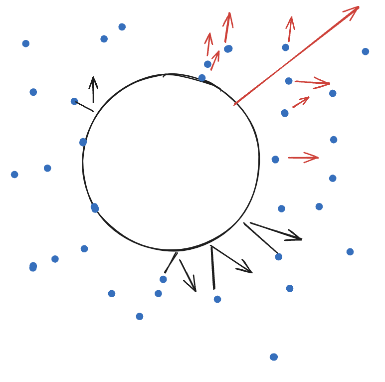
Kinetic theory model of Brownian particle. Notice how small and abundant the little particles are compared to the big one.
Let’s first adopt a macroscopic view of what’s happening here with full-on “ma = F”.
\[m \frac{d}{dt}\vec{v}(t) = -m \zeta \vec{v}(t)\]In this case, the term on the RHS is “force” and it should remind you of some sort of drag term. In hydrodynamics, this drag term is given by the Stokes drag equation $F_\text{drag} = 6\pi \eta R v$ so if we match up terms, this implies that $m \zeta = 6 \pi \eta R$. Plugging this back in, we can then solve the first order ODE, which just comes out to be an exponential decay solution.
\[m \frac{d}{dt}\vec{v}(t) = -6\pi \eta R \vec{v}(t)\] \[\vec{v}(t) = \vec{v_{0}}e^{-\zeta t}\]But there is something wrong with this “exponential-decay-to-zero” picture. Namely, we recognize that even when the BP is not being forced or dragged, it is never truly at rest because of the water molecules that constantly bombard it, kicking it around. In other words, to say that it has non-zero velocity on average, we can say that $\langle v^2 \rangle \neq 0$. We can update our picture by drawing something like the red squiggly line.
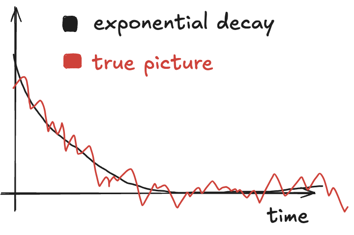
On average, there is an exponential decay (black). But there will always be nonzero fluctuations in velocity at thermal equilibrium, even when the velocity is '0' on average.
| When coupled to a thermal bath at equilibrium, we know by the [[20221013 Equipartition theorem states average kinetic energy equally shared among all degrees of freedom | equipartition theorem]] that each degree of free contains an energy contribution of $\frac{1}{2}k_{B}T$. For 3 degrees of freedom (in 3D space): |
To update our original differential equation, we need to add a random part, which turns it into a Stochastic Differential Equation.
\[m \frac{d}{dt}\vec{v}(t) = -m \zeta \vec{v} (t) + \vec{\eta}(t)\]But what exactly is this $\vec{\eta}(t)$ term that we have introduced (do not confuse it for the kinematic viscosity term from the Stokes drag equation). We can understand it from its statistical nature of its moments.
\[\begin{align} \langle \vec{\eta}(t) \rangle &= 0 \\ \langle \vec{\eta}_{i}(t) \vec{\eta}_{j}(t') \rangle &= 2 \Gamma \delta_{ij}\delta(t-t') \end{align}\]The first condition means that the ensemble average of all realizations of $\eta(t)$ trajectories is 0 for all t. The second condition is the correlation function condition, and it means that there is only nonzero correlation between two$\eta$ when you consider the same dimensions1 for infinitesimally short time lag $t=t’$.2
We are going to introduce a new variable $\vec{\Lambda}$ to normalize things nicely.
\[\begin{align} \vec{\Lambda}(t) &= \frac{1}{\sqrt{ 2 \Gamma }}\vec{\eta}(t) \\ \langle \Lambda_{i}(t) \Lambda_{j}(t) \rangle &= \delta_{ij}\delta(t-t') \end{align}\]After defining the Stochastic Differential Equation, we now need to solve it.
\[\vec{v}(t) = \underbrace{\vec{v}_{0}e^{-\zeta t}}_{\text{Homogeneous Solution}} + \frac{\sqrt{ 2\Gamma }}{m}\int_{0}^t d \tau e^{-\zeta (t-\tau)} \vec{\Lambda}(\tau)\]The second part of the RHS is the Green’s function perspective of solving inhomogeneous differential equations. In other words, another way of representing the “particular solution” is that it is the convolution of the impulse response $e^{-\zeta(t-\tau)}$3 with the “driving force” (the inhomogeneous part $\eta$, which we rescaled to $\Lambda$).
We analyze the correlation function for velocity and end up with
\[\begin{align} \langle v_{i}(t)v_{j}(t) \rangle = \underbrace{ v_{0,i}v_{0,j}e^{-\zeta(t+t')}\delta_{ij}\delta(\tau-\tau') }_{ \text{Homogeneous Part "Squared"} } + \underbrace{ \frac{2\Gamma}{m^2} \int_{0}^t d\tau \int_{0}^{t'} d \tau' \langle \Lambda_{i}(\tau) \Lambda_{j}(\tau')e^{-\zeta(t-\tau)}e^{-\zeta(t'-\tau')} }_{ \text{Inhomogeneous Part "Squared"} } \end{align}\]Notice that there are no cross terms here. This is because the ensemble average of the random variable $\Lambda$ with a constant is just 0, by definition of our Condition 1.
\[\begin{align} & \implies \frac{\Gamma}{\zeta m^2}e^{-\zeta|t-t'|}\delta_{ij} + \left( v_{0,i}v_{0,j}-\frac{\Gamma}{\zeta m^2}e^{-\zeta(t+t')} \right) \\ & = \frac{\Gamma}{\zeta m^2} \delta_{ij}e^{-\zeta |t-t'|} \end{align}\]We get to the last line by assuming that for $t,t’ \gg \zeta^{-1}$.
We can compare our solution to the Langevin equation with the known thermodynamic result regarding velocity correlations. Using the thermodynamic result and matching terms with our Langevin equation solution:
\[\langle v_{i}(t) v_{i}(t)\rangle = \frac{k_{B}T}{m}=\frac{\Gamma}{\zeta m^2}\]This means that
\[\boxed{ \Gamma = m \zeta k_{B}T \equiv \gamma k_{B}T }\leftarrow \text{Fluctuation-Dissipation Relation}\]Here we arrive at the Fluctuation Dissipation Relation. The amplitude of the noise is not so arbitrary. It is directly related to the viscous dissipation (friction) term on the macroscopic scale.
For a model of a particle in a fluid to be consistent with thermodynamics, it needs to be the case that
\[\begin{align} \frac{d}{dt}v_{i}(t) & = -m \zeta v_{i}(t) + \eta_{i}(t) \\ \langle \eta_{i}(t) \rangle& = 0 \\ \langle \eta_{i}(t) \eta_{j}(t') \rangle & = 2 \Gamma \delta_{ij} \delta(t-t') \end{align}\]with the constraint that $\Gamma = m \zeta k_{B}T$, which applies to systems coupled and in equilibrium with a thermal bath.
Stochastic dynamics of the displacement of a particle
Up until now, we’ve considered only the stochastic dynamics of the velocity of the particle, but what if we were interested in its position (or the distribution of positions). Below is the equation for the displacement of a particle from time = 0 to $t$. This is defined as integrating (accumulating displacements) velocity with respect to time from 0 to $t$.
\[\Delta x_{k}(t) = x_{k}(t) - x_{k}(0) = \int_{0}^{t}v_{k}(s)ds\]While the average displacement will equal 0 (since the particle can displace in any which direction just as likely as the other), we can instead consider a higher statistical moment, the average squared displacement.
\[\underbrace{ \langle |\Delta \vec{x}(t)|^{2}\rangle }_{ \text{MSD} } = \int_{0}^{t}d \tau \int_{0}^{t}d \tau' \langle \vec{v}(\tau)\vec{v}(\tau')\rangle\]After doing a lot of math (which I did not check), we end up with the formula
\[\text{MSD}= 2d \frac{k_{B}T}{m \zeta} \left[ t + \frac{1}{\zeta}(e^{-\zeta t}-1) \right]\]We can get an intuitive feel of this by considering the limits at very long and short time scales. When $t \gg \frac{1}{\zeta}$, we are in the diffusive regime:
\[\text{MSD} =\underbrace{ 2dDt }_{ x^{2} \sim t },\qquad \underbrace{ D=\frac{k_{B}T}{m \zeta} = \frac{k_{B}T}{6 \pi \eta R} }_{ \text{Stokes-Einstein} }\]But in the time regime where $t\ll \frac{1}{\zeta}$, we are in the ballistic regime (straight trajectory, too short of a timescale for any collisions to have happened).
\[\text{MSD} = \underbrace{ \frac{dk_{B}T}{m}t^{2} }_{ x^{2} \sim t^{2} }\]If you were to plot this as a function of MSD vs time in log-log, you’d end up with the two regimes being divided at the $t = \zeta^{-1}$ abscissa.4
Ballistic and diffusion regimes.
Recap
The reason why a microscopic fluctuation term and a macroscopic dissipation term are related to each other is because they come from the same microscopic origin of many particles (much smaller) bumping into the larger particle (or vice versa: larger particle bumping into many tiny particles).
-
meaning the spatial x, y, and z dimensions are independent of each other. ↩
-
Note that although both these are both $\delta$ symbols, one is the Kronecker Delta function and the other is the Dirac Delta function. The $\delta_{ij}$ is technically a tensor that that has the for the identity matrix. Only when the $i=j$ condition is met is the value equal to 1; otherwise, it is 0. The Dirac delta function $\delta(t-t’)$ is a continuous function of t, and is nonzero only when $\delta(0)$ or $t=t’$. It is a subtle and technical difference. ↩
-
The impulse response is also known as the homogeneous solution. Impulse response is the typical lingo for electrical engineers who’ve studied signals and systems. ↩
-
I’ve been wanting to use this word so badly. ↩