

Ostwald Ripening
September 18th, 2026
First pass of these notes. They are not very comprehendable because I barely comprehend these ideas myself yet. There are also missing media links. They are notes from Erwin Frey’s lectures on YouTube. I also think the presentation of these technical notes can be presented in a format other than an infinite scroll. Currently, the information is spaced out so widely that it’s easy to lose context. Something to think about for the future…
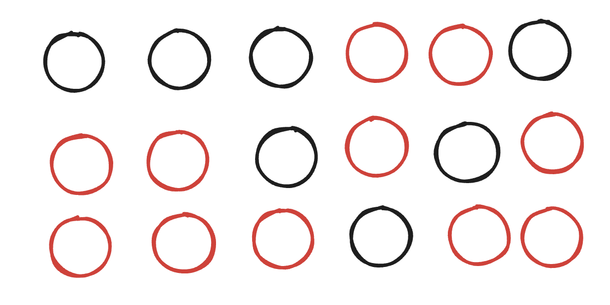
Lattice model of binary fluid mixture.
As always, we can define a Hamiltonian for a configuration of particles, which then in turn will help us define the partition function.
\[\mathcal{H}(\{\sigma_{i}\}) = \sum_{\langle i,j \rangle}\left[ \epsilon_{pp} \sigma_{i} \sigma_{j} + \epsilon_{ss}(1-\sigma_{i})(1-\sigma_{j}) + \epsilon_{ps}(\sigma_{i}(1-\sigma_{j})+\sigma_{j}(1-\sigma_{i}))\right]\] \[Z = \sum_{\{\sigma_{i}\}} \exp[-\beta \mathcal{H}(\{\sigma_{i}\})]\]Here, $\sigma$ can take on a value from 0 to +1, representing the black/red solutes. However, there are other formulations of this Hamiltonian where it takes a value from -1 to +1. $\epsilon$ is the nearest neighbor interaction coefficient with the solute and itself, the solute and the solvent, or the solvent with itself.
For the time being, let’s consider the scenario where there are no interaction energies (all the $\epsilon = 0$) other than site exclusion (one particle per site). Now, it becomes a matter of counting microstates. For a given number of solute and solvent particles, $N_p$ and $N_s$ respectively:
\[\Omega = \binom{N_{tot}}{N_{p}} = \frac{N_{tot}!}{N_{p}!N_{s}!}\]We are trying to calculate the entropy of the system (since there are no energetics with the absence of interaction terms, everything is entropically driven):
\[S = k_{B}\ln{\Omega}\]If we assume that we are dealing with a really big system ($N_p, N_s \gg 1$), then we can invoke Stirling’s Approximation, which will then yield the following form for entropy:
\[S = -N_{tot}k_{B}[\phi \ln \phi + (1-\phi)\ln(1-\phi)]\]where $\phi$ is the solute fraction $N_p / N_{tot}$ and ranges from 0 to 1. It is pretty easy to recognize that the distribution of the binary system that will maximize entropy is the one that is uniform, which in this case is 0.5/0.5 split between solute and solvent.
Now, let’s add back interactions. This makes the counting problem a lot harder. We can instead just coarse grain and jump to the mean-field theory. In doing this, we replace all local values by their spatial mean value $\phi$. We replace the microscopic Hamiltonian with a Hamiltonian that takes in $\phi$:
\[\mathcal{H}(\{\sigma_{i}\}) \rightarrow \mathcal{H}(\phi) \equiv E_{mf}(\phi)\] \[E_{mf}(\phi) = \frac{1}{2}zN[\epsilon_{pp}\phi^2 + \epsilon_{ss}(1-\phi)^2 + 2\epsilon_{sp}\phi(1-\phi)]\]where $z$ is just the number of neighbors each site has (in 2D, you have 4 neighbors; in 3D, you have 6 neighbors).
Now, we calculate the mean-field partition function:
\[Z_{mf} = \sum_{\{\sigma_{i}\}}\exp[-\beta E_{mf}(\phi)] = \Omega \exp[-\beta E_{mf}(\phi)]\]Note that because we have done a mean field, none of the terms explicitly depend on the configuration. It then just becomes a counting of microstates $\Omega$ that support that particular $\phi$.
\[F_{mf} = -k_{B}T\ln Z_{mf} = E_{mf}(\phi) - k_{B}T\ln \Omega\]We can rewrite the mean-field energy by collecting terms of $\phi$.
\[E_{mf}(\phi) = \frac{1}{2}zN[(\epsilon_{pp}+\epsilon_{ss}-2\epsilon_{ps})\phi^2 + c_{1}\phi+c_{0}]\]If you forgot where these equations come from, I will update them to clarify in the future (F = E - TS).
Moving along, we are more interested in energy differences than the magnitude of each state.
\[\Delta\epsilon \equiv \epsilon_{pp}+\epsilon_{ss}-2\epsilon_{ps}\]When $\Delta \epsilon < 0$, there is attraction between the solute and the solvent; when $\Delta \epsilon > 0$, there is repulsion.
We will now deal with the free energy density of a given patch.
\[f(\phi) = \frac{k_{B}T}{V}[\underbrace {\phi \ln \phi + ( 1 - \phi) \ln (1-\phi)}_{\text{Entropy Term}}+\underbrace{\chi \phi(1-\phi)}_{\text{Energy Term}}]\]Here we introduce a new term $\chi$, which is also known as the Flory-Huggins Parameter.
\[\chi = -\frac{z}{2}\frac{\Delta\epsilon}{k_{B}T}\]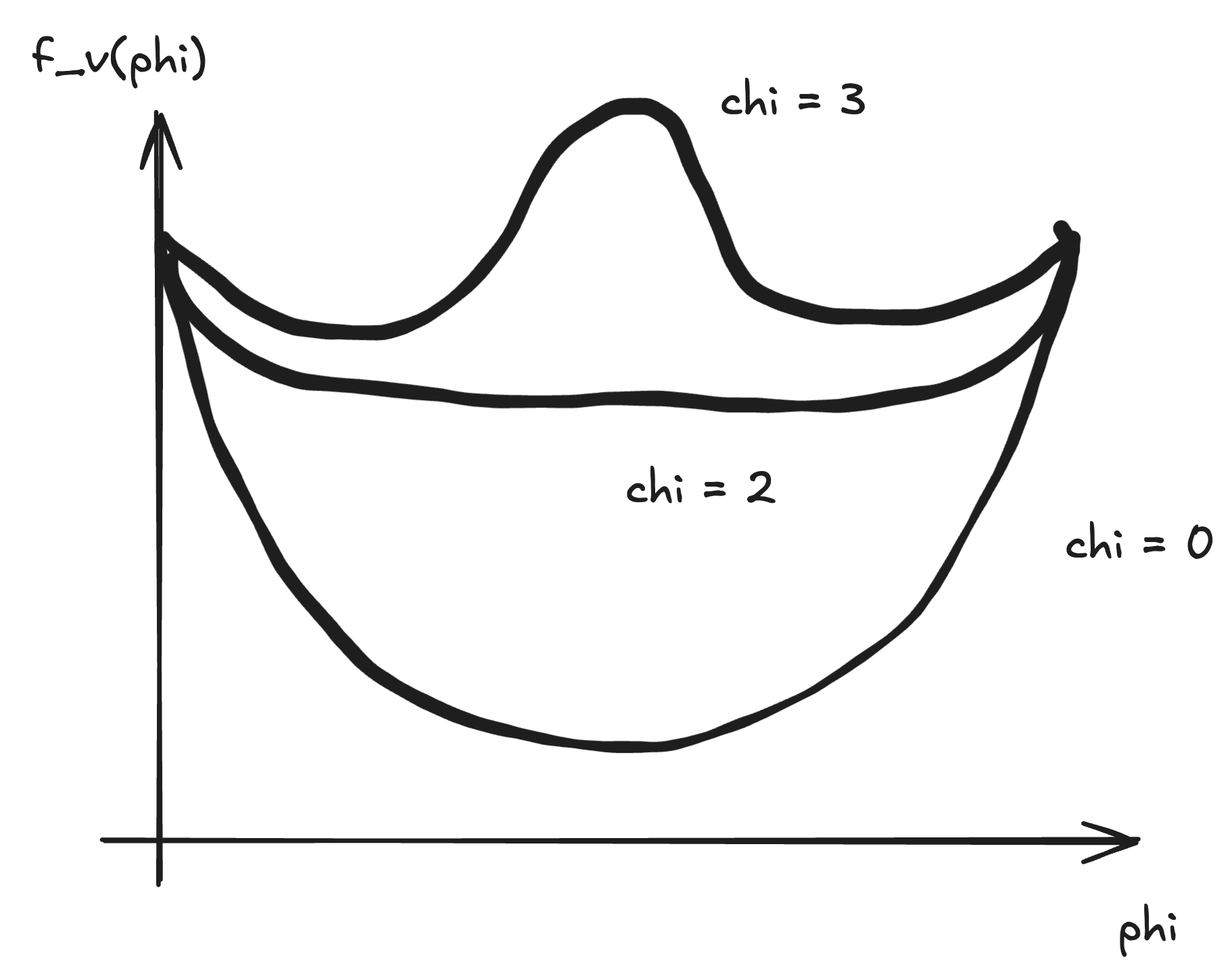
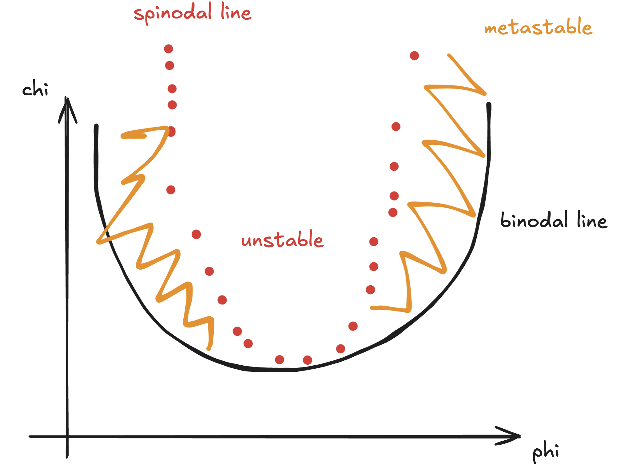
Here is an interesting phase diagram I’ve never seen before (usually it’s phi vs temperature). Since $\chi$ is a ratio of energy:temperature, a greater $\chi$ means that the energetic attraction is a bigger effect than temperature fluctuations. This energetic favorability can induce demixing, which makes sense that it can drive a given value of $\phi$ into the binodal and spinodal lines.
Spatial heterogeneity
We will now try to figure out a mean-field theory that can account for spatial heterogeneities. In the previous section, it was only concerned with the thermodynamic equilibrium where things have coarsened completely to just two domains.
The microscopic Hamiltonian will go from being a discrete-configuration definition to an integral defined as so:
\[\mathcal{H}(\{\sigma_{i}\}) \rightarrow \chi k_{B}T\int \frac{d^3r}{V} \frac{a^2}{2} (\nabla \sigma(\vec{r}))^2\]We come to this form by recognizing that there is rotational invariance (the energy of the system should not depend on the orientation as you rotate). What does contribute are the gradients or boundaries. Now, instead of defining a solute/solvent at a site, we define its spatial average at a position after coarse-graining.
This leads to the following Ginzburg-Landau Free Energy Functional. It is a functional because it takes in as input the 2D scalar function $\phi(\vec{r})$ and outputs the energy for that particular landscape configuration.
\[F[\phi(\vec{r})] = \int d^3 \vec{r}\left[ f(\phi) +\frac{c}{2}(\nabla \phi)^2 \right]\]The first term is the energy density of the patch at that point. The second term is the energy term from the $c \sim k_{B}T\chi$.
After defining this Free Energy Functional, we get the Partition Function, which is defined as an integral over the function space of $\phi(\vec{r})$, which can be any possible landscape that respects the boundary conditions and any other constraints.
\[Z = \int D[\phi(\vec{r})]\exp[-\beta F[\phi(\vec{r})]]\]Recall that $f(\phi)$ has logarithm terms, so if we don’t want to deal with that, we can instead expand about the threshold.
\[BF[\phi] = \int \frac{d^3 \vec{r}}{V}\left[ (2-\chi)\delta \phi^2 + \frac{4}{z}(\delta \phi)^4 + \frac{1}{2} \tilde{\kappa}(\nabla\delta \phi)^2 \right]\]This is a very similar phenomenological equation as that of the Ising Model.
We are going to define another order parameter called particle density $c \equiv \frac{\phi}{V}$ (aka concentration, but I need to check this[^1]) and this allows us to rewrite the equation (after dividing through by $V$). You’ll notice that the first two terms are the local terms and result in a 4-th order well (two wells to be precise) while the third term is the gradient term.
\[F = \int d^3 r \left[ -\frac{1}{2}r(c-c_{c})^2 + \frac{1}{4}u(c-c_{c})^4 + \frac{1}{2} \kappa (\nabla c)^2 \right]\]We are now ready to define interface and surface tension. Consider that the concentration profile is constant at negative and positive infinity. When this profile is established, we are at thermodynamic equilibrium and the change of free energy with respect to concentration profile is 0: $\frac{\delta F}{\delta c} = 0$. This is essentially taking the (functional) derivative of Free energy and seeing for what concentration landscape $c(x)$ is it minimal? That is where $\frac{\delta F}{\delta c} = 0$.
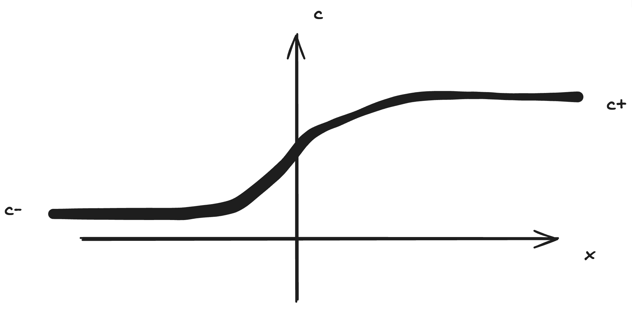
If we actually go through with taking this functional derivative, we see that:
\[\frac{\delta F}{\delta c} = f'(c) - \kappa \partial_{x}^2\tilde{c}=0\]This is made clearer by direct application of the Euler-Lagrange Equation (but instead of considering the derivative of the action functional, we are considering the derivative of the free energy functional):
\[\frac{\delta F}{\delta c} = \frac{\partial f(c)}{\partial c} + \frac{\partial(\kappa (\nabla c)^2/ 2)}{\partial (\nabla c)}\]What this equation with the Laplacian and the $f’(c)$ term tells us, given that $f(c)$ is our double well function is that the solution is the classic hyperbolic tanh function. Since the coarse-grained Ising model has a double-well potential as well, it also gives rise to the tanh function at the boundary between two phases. Even when we get to the Cahn-Hilliard section where the interfaces are all work-like an bubbly, if you zoom into the boundaries between the two phases, they will look like tanh.
\[\tilde{c}(x) = c_{c} + \sqrt{ \frac{r}{u} } \tanh{\frac{x}{\xi}}\]where $r$ and $u$ are phenomenological parameters.
Cahn-Hilliard Dynamics
Finally, we will talk about Cahn-Hilliard dynamics. It is unique from, say, an Ising system or Allen-Cahn system, in that it conserves mass.[^2] With conservation, you have the following form:
\[\partial_{t}c(\vec{r},t) = -\nabla \cdot \vec{J}(\vec{r},t)\]This basically says that the change in concentration in a location depends on the divergence of current at that spot. The current itself is defined by the gradient of a chemical potential, which can be recognized from Onsager reciprocal relations, which relates gradients of potentials to currents.
\[\vec{J}(\vec{r},t)=-\lambda(c) \nabla \mu(\vec{r},t)\]In this case, the chemical potential is defined as $\frac{\partial F[c]}{\partial c}$. Let’s take a moment to understand this. When you take the derivative of an energy (thermodynamic potentials like internal energy, Gibbs, enthalpy, and Helmholtz), with respect to one conjugate variable, you’ll get the other conjugate variable. The thermodynamic conjugate variable to concentration (or particle number in discrete systems) is chemical potential.
So when we think about conservation of mass in this system, we’ll be looking at the currents from the gradients in chemical potential.
\[\frac{\partial F[c]}{\partial c} = f'(c(\vec{r},t))-\kappa \nabla^2 c(\vec{r},t)\]When we plug this into the differential equation for concentration, we get that
\[\partial_{t}c(\vec{r},t)=\nabla \cdot (\lambda(c) \nabla[f'(c) - \kappa \nabla^2 c])\]We can pull out $\lambda(c)$ if we linearly expand it about the stable concentration field $c_c$.
\[\partial_{t}c(\vec{r},t) = \lambda(c_{c}) \nabla^2 [f'(c) - \kappa \nabla^2 c]\]We can now do linear stability analysis about the homogeneous concentration field to see how it becomes unstable.
\[c(\vec{r},t) = \bar{c} + \delta c(\vec{r},t)\]We will insert this into the differential equation and keep only the linear terms (the constant terms contribute 0 to the time dynamics; higher order terms we will neglect since this is linear stability analysis)
\[\partial_{t} \delta c(\vec{r},t) = \lambda(\bar{c}) \nabla^2 [f''(\bar{ c})\delta c(\vec{r},t)-\kappa \nabla^2\nabla c(\vec{r},t)]\]This makes sense since for $f’(\bar{c} + \delta c) \sim f’(\bar{c})+f’’(\bar{c})\delta c \dots$.
Since we only have time derivatives and spatial derivatives, the time is ripe to do Fourier analysis. Assuming the solution takes the form of superposition of Fourier modes:
\[\delta c(\vec{r},t) = \int d^dk \ \delta c(\vec{k}, t)e^{i \vec{k} \cdot \vec{r}}\]We examine the dynamics of a single mode by plugging it into the differential equation for a given $\vec{k}$:
\[\partial_{t} \delta c(\vec{k},t) = \sigma(\vec{k}) \delta c(\vec{k},t)\]where the amplification factor $\sigma$ takes the form:
\[\sigma(\vec{k}) = -\lambda(\bar{c})k^2[f''(\bar{c})+\kappa k^2]\]where we can see that we just replaced any nablas with the wavenumber $k$. When we plot this, we end up getting:
In the case that we are on a point of the double-well free-energy density function that is concave up (like the dips of the wells themselves), the system is considered stable to infinitesimally small perturbations (like thermal fluctuations). But we are on the part of the function that is concave down, then we are in the unstable regime, and the mode $k_{max}$ will be the quickest growing mode we’ll see first.
Nonequilibrium dynamics of the droplets with classical nucleation theory
Given that we are in the metastable regime, what is the minimum size droplet that will grow? (rather than quickly shrink back into the mixed state).
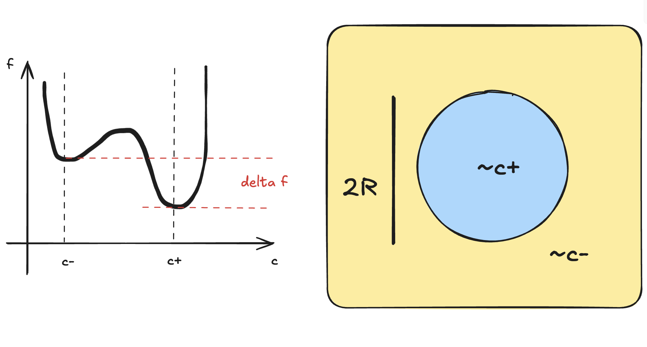
What is the energetic cost (and benefit) of creating such a droplet depends on the energetic difference between the pure c- and the c+ state (in this case, it is energetically favorable) $\Delta f$. However, there will always be the cost of creating an interface between the two phases. This will incur an interface energy penalty.
\[\Delta F = \Delta f \frac{4}{3}\pi R^3 + \gamma4\pi R^2\]where the $R^3$ term is the volumetric energy difference density and the $R^2$ is the interfacial energy penalty.
Assuming that the droplet phase is more stable $\Delta f < 0$. There is a competition between favoring the droplet as $R^3$ and fighting against the droplet as $R^2$.
![[ostwald-critical-droplet-radius]]
There is a critical droplet radius. Before that radius, there is an activation barrier to overcome. Beyond the critical radius, it is favorable to keep growing until you enter the other regime (where you have worms instead of droplets). This is the same energy barrier that must be overcome when you are in the concave negative part of the energy diagram (and in the metastable part of the phase diagram).
When we are at thermodynamic equilibrium, the chemical potential is equal everywhere — there are no gradients in chemical potential (there can be gradients in concentration though) so there is no net flux of molecular species[^3]. That means at an interface, the chemical potential is equal on both sides. But recall that for curved interfaces, there will always be a [[20240716 Laplace pressure]]. We thus have to balance the mechanical work with the interfacial work for an increase in radius $dR$.
\[P_{\gamma}4\pi R^2 dR = 4\pi[(R+dR)^2 - R^2]\gamma\]This reveals to us that the Laplace pressure is related to the interfacial tension by
\[P_{\gamma} = \frac{2\gamma}{R}\]Yes, chemical potential $\mu_{in}=\mu_{out}$, but what is balancing the mechanical Laplace pressure? This is where we introduce (and motivate) the idea of osmotic pressures. There is an osmotic pressure on the inside and on the outside.[^4]
\[\Pi_{in} = \Pi_{out} + \frac{2\gamma}{R}\]We consider a small variation $\delta c_{in}$ and $\delta c_{out}$ to consider stability about the equilibrium.
\[c_{in} = c_{+} + \delta c_{in}\] \[c_{out}= c_{-}+\delta c_{out}\] \[f_{in}=f(c_{in}) \sim f(c_+)+\frac{1}{2}f''(c_{+})\delta c_{in}^2\] \[f_{out}=f(c_{out})\sim f(c_{-})+\frac{1}{2}f''(c_{-})\delta c_{out}^2\]Because we are expanding about the bottom of the double wells, the slope $f’$ is 0 there so the first non-zero term after the constant is the $f’’$ term.
Remember, the chemical potentials are equal in and out. And recall that $\mu = \frac{\partial f}{\partial c}$, which is where the idea of common tangency comes in. So when we take the derivative of $f_{in}$ and $f_{out}$ with respect to $\delta c$, then we get:
\[f''(c_{+})\delta c_{in}=f''(c_{-})\delta c_{out}\]For an ideal mixture, this double well will also have the same concavity upwards (each thing likes itself just as much).
\[\delta c_{in} = \delta c_{out}\]This means that for any disturbance from equilibrium, any changes in droplet internal concentration will result in a change in external concentration.[^5]
Now, we have to consider the difference in osmotic pressure to wrap up our discussion of mechanical equilibrium with Laplace pressure. Recall from [[20260831 Osmotic pressure is negative pressure]] derivation that $\Pi_{in} = \mu_{in}c_{in}-f_{in}$.
\[\Pi_{in} - \Pi_{out} = f''(c_{\pm})(c_{+} - c_{-}) \delta c\]Plug this osmotic pressure difference into the equation that relates Laplace and osmotic pressure at mechanical equilibrium. We will generalize from 3-dimensions to $d$ dimensions.
\[\begin{align} \Pi_{in} - \Pi_{out} &= \frac{\gamma}{R} (d-1) \\ \delta c &= \frac{d-1}{(c_{+} - c_{-})f''(c_{\pm})} \frac{\gamma}{R} \end{align}\]This is the famed Gibbs-Thomson Relation, which relates the difference in concentration across a curved surface with positive interfacial energy. As you can see, when you make the droplet bigger (increase $R$), then the variation in concentration from the $c_{\pm}$ minima decreases ($\delta c$ decreases). As you increase the surface tension $\delta c$ increases. And as you make the energy wells wider (decrease $f’‘(c_\pm)$), then $\delta c$ increases.
Another way to write the Gibbs-Thomson relation is to do so as a ratio of length scales, namely the capillary length scale and the radius of the droplet.
\[\begin{align} l_{\gamma}^\pm &= \frac{(d-1)\gamma}{(c_{+} - c_{-})c_{\pm}f''(c_{\pm})} \\ \delta c &= c_{\pm}\frac{l_{\gamma}^\pm}{R} \end{align}\]Dynamics of a single droplet
Let us recognize that we are in a supersaturated regime. The width of the droplet, $\xi « R$, where $R$ is the size of the system. We make this assumption because it allows us to make a separation of length scales argument. The width of the droplet interface (inside and outside transition length) is much smaller than the size of the system itself and appears seemingly “sharp”. ![[20251126 Ostwald ripening 2026-09-17 14.15.16]] We end up with the situation that:
\[\begin{align} \partial_{t}c(\vec{r},t) &= \nabla \cdot [\lambda(c) f''(c) \nabla c(\vec{r},t)] \\ &= \nabla \cdot [D_{eff}(c) \nabla c(\vec{r},t)] \end{align}\]As opposed to last time, the $\kappa$ term is not neglected in the ==sharp interface limit== because we are interested in the flat outside bulk.
What is the steady state profile $\partial_t c = 0$? Recognize the separation of time scales of this problem. The change in radius is slow dynamics while the change in concentration is a fast dynamics thing.
To solve this problem, we first consider and uphold the boundary conditions. Start with Laplace’s equation:
\[\nabla^2 c(r) = 0\implies \frac{1}{r^2}\partial_{r}r^2 c(r) = 0\]where the second equation is Laplace’s equation in spherical coordinates, which is convenience when considering the sizes of spheres.
We have the boundary conditions of the droplet that the derivative of concentration at the center of the droplet is 0, $\partial_{r}c(r)\vert_{r=0} = 0$, the concentration very far away from the droplet is $c_\infty$ and the concentration right at the boundary of the droplet is $c_{out}$
![[20251126 Ostwald ripening 2026-09-17 14.39.00]]
In the case that the interface moves (for reasons like growing or shrinking of droplet), we need to conserve mass of the chemical species.
\[(c_{in}-c_{out})\partial_{t}R = J(r)|_{r=R_{-}} - J(r)|_{r=R_{+}}\]The term on the right hand side is the difference in flux at the boundary, and it causes the boundary interface to move. Notice that the concentration profile is flat on the inside of the droplet, which means that there is no flux on the inside surface. There is, however, just on the outside of the droplet.
\[\vec{J}(r) = -\lambda \nabla \mu \sim -\lambda f''(c_{-})\nabla c\] \[\vec{J}(r) = -\lambda f''(c_{-})\hat{\vec{n}}\partial_{r}(c(r))\]Given that the droplet is radially symmetric, you will get
\[J(r=R_{+}) = \lambda f''(c_{-})(c_{out} - c_{\infty}) \frac{1}{R}\]Plugging this back to solve for $\partial_t R$, we get the following equation for how the radius of the droplet will change over time.
\[\partial_{t}R = \frac{\lambda f''(c_{-})}{c_{+}-c_{-}} \cdot \frac{\epsilon - \delta c(R)}{R} = \frac{\lambda f''(c_{-})}{c_{+} - c_{-}} \frac{1}{R} \left( \frac{\epsilon}{c_{-}} - \frac{l_{\gamma}^-}{R} \right)\]Setting the derivative to 0 gives us a steady state radius, a radius at which the droplet will not grow or shrink.
\[R^* = l_{\gamma}^- \frac{c_{-}}{\epsilon}\]Doing stability analysis graphically:
![[20251126 Ostwald ripening 2026-09-18 14.35.39]]
We see that the equilibrium point is not stable. It will either grow much bigger, entering a new regime beyond droplet growth (can become worms and stuff) or it will shrink back down and vanish.
Considering collectives of droplets
Up until now, we’ve only considered the dynamics of a single droplet. But what if there are many droplets of various sizes. And what if they are sharing the same global reservoir of material?
This will probably be a discussion for another day,